Quantifying Restoration: PSNR, SSIM, and Morphology in Deep-Learned Galaxies

Table of Links

Abstract and 1 Introduction

2 Method

2.1. Overview and 2.2. Encoder-Decoder Architecture

2.3. Transformers for Image Restoration

2.4. Implementation Details

3 Data and 3.1. HST Dataset

3.2. GalSim Dataset

3.3. JWST Dataset

4 JWST Test Dataset Results and 4.1. PSNR and SSIM

4.2. Visual Inspection

4.3. Restoration of Morphological Parameters

4.4. Restoration of Photometric Parameters

5 Application to real HST Images and 5.1. Restoration of Single-epoch Images and Comparison with Multi-epoch Images

5.2. Restoration of Multi-epoch HST Images and Comparison with Multi-epoch JWST Images

6 Limitations

6.1. Degradation in Restoration Quality Due to High Noise Level

6.2. Point Source Recovery Test

6.3. Artifacts Due to Pixel Correlation

7 Conclusions and Acknowledgements

Appendix: A. Image restoration test with Blank Noise-Only Images

References

4. JWST TEST DATASET RESULTS

In this section, we present the results when our deep learning model is applied to the JWST test dataset. We first define the two evaluation metrics: peak signal-to-noise ratio (PSNR) and structural similarity index measure (SSIM), describe our visual inspection, and compare morphological and photometric properties.

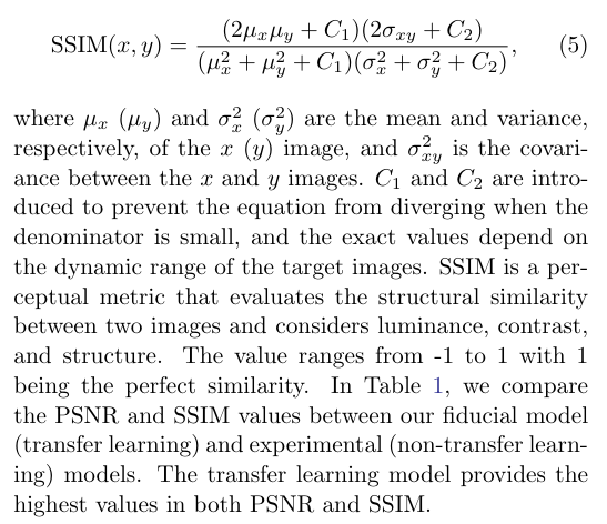
4.1. PSNR and SSIM

The PSNR and SSIM metrics are employed to evaluate the similarity between LQ and GT images and guide the selection of our best models. The mean squared error (MSE) is defined as:

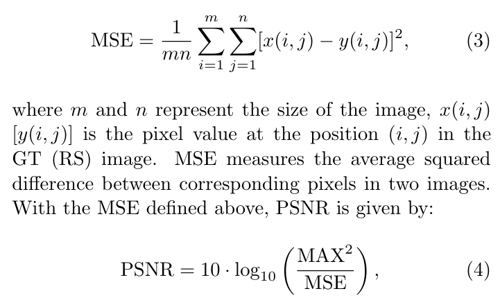
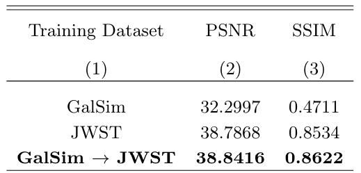
Table 1. Comparison of PSNR and SSIM performance between the model trained through transfer learning and the models trained with either the GalSim or JWST dataset.

where MAX is the peak value of the GT image. Compared to MSE, PSNR takes into account the image-byimage difference in peak values.

The SSIM metric is defined as:

4.2. Visual Inspection

Figure 5 shows several image restoration cases in ascending order of rms noise level. We select examples, which have rich substructures, low-surface brightness features, and extended morphologies. The visual inspection indicates remarkable improvements in both resolution and noise level. Detailed substructures such as starforming clumps and spiral arms have been restored with high fidelity. Also, the restored overall morphological features such ellipticity and core size are consistent with those of the GT images. In addition, the low-surface brightness edges are restored remarkably well. Finally, we note that the performance is not very sensitive to the input noise level, which in this example varies by a factor of 3.

4.3. Restoration of Morphological Parameters

Although one can characterize galaxy morphologies in various ways, we employ best-fit Sersic parameters to quantify the comparison. Specifically, we compare the two ellipticity components: e1 and e2, Sersic index n, half-light radius R50, and the intensity at R50.

The two components of the ellipticity are motivated by the weak lensing convention, which utilizes not only the absolute ellipticity e of a galaxy but also its position angle θ as follows:

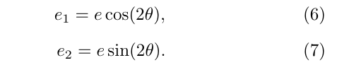
The ellipticity e is defined as (a − b)/(a + b), where a and b are the semi-major and -minor axes, respectively.

Figure 6 compares the five morphological parameters. Across all parameters, the RS images exhibit stronger correlations with the GT images in terms of the scatter and slope of the correlations. The ellipticity comparison shows that the LQ galaxies are systematically rounder than the GT galaxies, which is not surprising because they are generated by convolving the GT galaxies with the circular HST PSF. This bias nearly disappears in the RS images. The improvement in the Sersic index n is remarkable. The scatter is reduced by more than a factor of 3. Also, the Pearson correlation coefficient improves from 0.61 to 0.90. Given that the Sersic index n is one of the most difficult parameters to restore, its recovery showcases the stability of the restoration performance. The R50 recovery is also noteworthy with the reduction of the scatter by more than a factor of 4 and the increase of the Pearson correlation coefficient by ∼48%. Finally, the I(R50) intensity comparison shows a scatter reduction of ∼46% and an increase of the correlation by ∼9%.

4.4. Restoration of Photometric Parameters

One of the immediate scientific utilities of image restoration is enhancing photometry. Here we compare aperture flux, isophotal flux, and individual pixel values measured from the RS images with the GT images to evaluate the performance in the photometric context.

Since we use min-max normalization consistently across our training and input datasets, the dynamic range of the RS images is also restricted. To extract photometry from the LQ and GT images, we opt to use the original (pre-normalization) images. Consequently, it is necessary to rescale the RS images. To ensure a fair comparison, this rescaling process must be executed independently, without relying on the information available from the corresponding GT images.

We aligned the dynamic range of the RS images to the LQ images as follows. First, we measured the lower

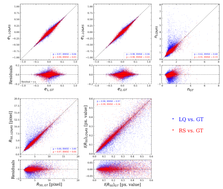
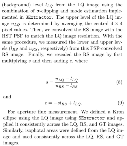
Figure 7 displays the resulting flux comparisons. The aperture fluxes from the RS images are in good agreement with those from the GT images. Compared to the LQ images, the scatter is reduced by ∼60%. The scatter reduction is similar (∼55%) in isophotal flux. It is

worth noting that the isophotal fluxes in the LQ images are systematically overestimated because the isophotal area is defined from the LQ image[5]. This bias is significantly reduced in the RS images. Finally, the pixel-to-pixel comparison illustrates a tight 1:1 correlation between the RS and GT images across the entire dynamic range, while the LQ images show a slope significantly less than unity because of their larger PSF. The pixel-to-pixel scatter reduction is by a factor of 7.

[5] That is, noise can make some pixel values near the edge of the isophotal area in the LQ image higher than the GT values.